Some preliminary definitions

First, we introduce the ring we will be working in. Here I will use $$R = \mathbb{C}[x_1 , \dots , x_n] \, , $$ the polynomial ring in $n$ variables with complex coefficients. This is a nice ring: it is Noetherian, which means that every ideal $I$ if $R$ is finitely generated. Moreover, the base field $\mathbb{C}$ is algebraically closed, which will be important at some points of the discussion.

Now we need to introduce a concept analogous to the prime numbers in the fundamental theorem of arithmetics. However we will see that two related but distinct notions are required:

• An ideal $I$ is called prime if $fg \in I$ implies either $f \in I$ or $g \in I$.
• An ideal $I$ is called primary if $fg \in I$ implies either $f \in I$ or $g^m \in I$ for some integer $m>0$.

• An ideal $I$ is called radical if $f^m \in I$ for some integer $m>0$ implies implies $f \in I$.

The importance of radical ideals comes in part from the fact that they are the ideals that correspond to varieties. If $V \subset \mathbb{C}^n$ is a variety, then the vanishing ideal $\mathcal{I}(V)$ is radical, and more importantly (and here we use the fact that $\mathbb{C}$ is algebraically closed), we have the Nullstellensatz $$\mathcal{I}(\mathcal{V}(I)) = \sqrt{I} \, , $$ where $\mathcal{V}(I)$ is the variety defined by the ideal $I$. We will come back later to the connection between ideals and varieties, in relation to the decompositions of ideals, to which we turn now.

Ideal decompositions

Prime decomposition

We begin with the theorem of prime decomposition. Here we use the fact that $\mathbb{C}$ is algebraically closed. The theorem of prime decomposition tells us that any radical ideal $I \subset R$ can be written uniquely as a finite intersection of prime ideals $$I = P_1 \cap \dots \cap P_r$$ with $P_i \not\subset P_j$ for $i \neq j$.

The crucial assumption in the previous theorem is the fact that $I$ must be radical. Note that, as we said above, this is always satisfied if $I = \mathcal{I}(V)$ is the vanishing ideal of a variety. In the next section, we state a theorem that gives a decomposition for any (not necessarily radical) ideal.

Primary decomposition

We now state the main theorem of this note, called the principal decomposition theorem, of the Lasker-Noether theorem (note that Emanuel Lasker is maybe more well-known today for his career as a chess player: he reined as World Chess Champion for 27 years, more than any other World Chess Champion, and he is regarded as one of the strongest players of all times).

Any ideal $I \subset R$ has a decomposition $$I = Q_1 \cap \dots \cap Q_r$$ where the $Q_i$ are primary ideals, the prime ideals $P_i = \sqrt{Q_i}$ are all distinct and $\cap_{j \neq i} Q_j \not\subset Q_i$ for all $i$. Moreover, the $P_i$ are uniquely determined, and are called the associated primes (but the $Q_i$ are not uniquely determined in general).

The above theorem is also true if the base field $\mathbb{C}$ is replaced by an arbitrary (not necessarily algebraically closed) field. Also, there is a slightly stronger result concerning the unicity: the $Q_i$ associated to a minimal prime $P_i$ (in the sense that no $P_j$ is strictly contained in $P_i$) is uniquely determined. In the ring of integers, the minimal prime ideals over a nonzero ideal $\langle m \rangle$ are the ideals $\langle p_i \rangle$ where the $p_i$ are the prime divisors of $m$. This means that in the primary decomposition of $\langle m \rangle$, the primary ideals (which correspond to powers of the primes $p_i$) are uniquely determined -- this is the fundamental theorem of arithmetics!

As we see, the primary decomposition is almost unique, in the sense that we have some degree of freedom in the choice of the $Q_i$, but only among the primary ideals whose radical correspond to the uniquely determined prime ideals $P_i$ that are not minimal.

Let's give an example. Consider in $R=\mathbb{C}[x,y]$ the ideal $I = \langle x^2 , xy \rangle$. Then the associated primes are $P_1 = \langle x \rangle$ and $P_2 = \langle x,y \rangle$. Note that $P_1 \subset P_2$, so $P_1$ is minimal but $P_2$ is not. This means that in primary decompositions of $I$, the primary ideal $Q_1$ will be uniquely determined, but not the primary ideal $Q_2$. Indeed, we find that for any integer $m>0$, a primary decomposition of $I$ is $$I = \langle x \rangle \cap \langle x^2 , xy , y^m \rangle \, . $$

The relation with geometry

Let $V \subset \mathbb{C}^n$ be an affine variety. Then $V$ is irreducible if and only if the ideal $\mathcal{I}(V)$ is a prime ideal. We have the following result, which mirrors the prime decomposition of ideals: if $V \subset \mathbb{C}^n$ is an affine variety, then it has a unique decomposition $$V = V_1 \cup \dots \cup V_r$$ where the $V_i$ are irreducible and $V_i \not\subset V_j$ for $i \neq j$. Furthermore, this decomposition is unique up to the order in which the $V_i$ are written.

Now let's turn to the primary decomposition of ideals. The decomposition $$I = Q_1 \cap \dots \cap Q_r$$ defines a decomposition $$\mathcal{V}(I) = \mathcal{V}(Q_1) \cup \dots \cup \mathcal{V}(Q_r) = \mathcal{V}(P_1) \cup \dots \cup \mathcal{V}(P_r) \, , $$ where we have used the fact that $\mathcal{V}(P_i) = \mathcal{V}(Q_i)$. In fact, one can even write (as far as algebraic varieties are concerned -- i.e. not schemes) $\mathcal{V}(I)$ as the union of the $\mathcal{V}(P_j)$ where the $P_j$ are the minimal primes.

Let's illustrate that with our example above. To the ideal $I = \langle x^2 , xy \rangle$ is associated the line of equation $x=0$. In the decomposition of that variety given by the primary decompositions above, we have the two varieties $\mathcal{V}(P_1) = \{x=0\}$ and $\mathcal{V}(P_2) = \{x=y=0\}$. We see that $P_1 \subset P_2$ translates into $\mathcal{V}(P_2) \subset \mathcal{V}(P_1)$, as expected, and we can remove the component $\mathcal{V}(P_2)$ from the union.

In summary, although the primary decomposition is not unique, the corresponding decomposition in terms of varieties is unique, and is given by the mininal prime ideals among the radical of the primary ideals present in any primary decomposition.

References

• Cox, David, John Little, and Donal O'shea. Ideals, varieties, and algorithms. Vol. 3. New York: Springer, 2007. In particular, chapter 4.
• Wikipedia article on primary decomposition.

Il n'est pas difficile de faire l'application numérique : on trouve $$5000000 \frac{h \alpha}{c e^2} = 3,14159265 \, \textrm{m}.\textrm{kg}.\textrm{s}^{-2}.\textrm{A}^{-2} \, . $$ On reconnaît évidemment le nombre $\pi$. Mais cette valeur est-elle exacte ? Et cette question de l'exactitude d'une constante physique a-t-elle un sens ?

En fait, il se trouve que la quantité ci-dessus est, à une constante entière près, égale à la perméabilité magnétique du vide $\mu_0$, et c'est cette grandeur qui sert à définir l'ampère. Plus précisément, la seconde, le mètre et le kilogramme ayant été définis préalablement, on définit l'ampère par la relation $$\mu_0 = 4 \pi \times 10^{-7} \, \textrm{m}.\textrm{kg}.\textrm{s}^{-2}.\textrm{A}^{-2} \, . $$ Et comme par définition de la constante de structure fine, $\mu_0 = \frac{2 h \alpha}{c e^2}$, on obtient bien $$5000000 \frac{h \alpha}{c e^2} = \pi \, \textrm{m}.\textrm{kg}.\textrm{s}^{-2}.\textrm{A}^{-2} \, . $$ C'est une valeur exacte.

Il faut noter que dans le SI, ni la constante de Planck $h$, ni la charge de l'électron $e$, ni la constante de structure fine $\alpha$ ne sont définies comme des valeurs exactes. Toutes dépendent d'expériences réalisées pour les déterminer, dans un système d'unités donné à l'avance par d'autres définitions (la vitesse de la lumière, elle, est définie exactement, $c=299792458 \, \textrm{m}.\textrm{s}^{-1}$). Il est amusant de voir que ces incertitudes "conspirent" pour donner une valeur exacte (même si évidemment, il n'y a rien de remarquable à cela : par exemple la constante de structure fine $\alpha$ conspire également avec $\pi - \alpha$ pour donner une somme égale à $\pi$).

Ce qui est plus amusant est de remarquer que cet état de fait va bientôt changer. En effet, prochainement la définition des unités SI devrait être modifiée (voir par exemple cet article Wikipedia). La définition de la seconde n'est pas modifiée, celle du mètre non plus (ainsi la valeur exacte de $c$ perdure), mais les définitions du kilogramme et de l'ampère se feront en termes de $h$ et $e$ respectivement. Autrement dit, ces deux valeurs seront alors parfaitement exactes dans le nouveau système SI. En revanche, $\mu_0$ perdra son statut de constante exacte. Il est amusant de voir que dans le rapport $\frac{h \alpha}{c e^2}$, on passera donc de une à trois constantes exactes, mais que sa valeur cessera d'être exacte.

Bref, ce petit calcul était l'occasion de mentionner cette prochaine modification des définitions du SI (voir aussi sur le blog de David Madore ici) et de susciter la réflexion sur ce que signifie être exact pour une grandeur physique.

The geometry of orbits

In all the following we fix a quiver $\vec{Q}$, and we will drop the $\vec{Q}$ dependence although of course all the construction depends on $\vec{Q}$. Let $V$ be a finite-dimensional representation of $\vec{Q}$, with dimension vector $\mathbf{v}$ (see the first post for definitions and notations). When the dimension is fixed, we can assume the vector spaces at nodes of the quiver are just $\mathbb{C}^{\mathbf{v}_i}$, and the particular representation $V$ is specified by the matrices of the various linear maps corresponding to the edges. Let's call $$R( \mathbf{v}) = \bigoplus\limits_{h \in \Omega} \mathrm{Mat}_{\mathbf{v}_{t(h)} \times \mathbf{v}_{s(h)}}(\mathbb{C})$$ the representation space. The group $$\mathrm{PGL}( \mathbf{v}) = \left( \prod\limits_{i \in I} \mathrm{GL}( \mathbf{v}_i) \right) / \mathbb{C}^{\ast}$$ acts on $R( \mathbf{v})$ by conjugation, and two elements of $R( \mathbf{v})$ define isomorphic representations if and only if they are in the same $\mathrm{PGL}( \mathbf{v})$ orbit. So, in other words, the isomorphism classes of representations $V$ of dimension $\mathbf{v}$ are the $\mathrm{PGL}( \mathbf{v})$ orbits $\mathbb{O}_V$ in $R( \mathbf{v})$.

Now we can state an important result: the orbit $\mathbb{O}_V$ is closed if and only if $V$ is semisimple, and the closure of any $\mathbb{O}_V$ contains a unique closed orbit, namely $\mathbb{O}_{V^{\mathrm{ss}}}$.

These facts should resonate with the GIT theory! Indeed, these can be reformulated as $$R( \mathbf{v})/\mathrm{PGL}( \mathbf{v}) = \{\textrm{Isomorphism classes of reps of dimension } \mathbf{v}\}$$ $$\mathcal{R}_0 ( \mathbf{v}) := R( \mathbf{v})// \mathrm{PGL}( \mathbf{v}) = \{\textrm{Isomorphism classes of semisimple reps of dimension } \mathbf{v}\} \, . $$ Finally, this begs for the introduction of twisted GIT quotients. For that, note that the characters of $\mathrm{PGL}( \mathbf{v})$ are of the form $$\chi_{\theta} : g \mapsto \prod\limits_{i \in I} \det (g_i)^{- \theta_i} \qquad \textrm{with} \qquad \theta \in \mathbb{Z}^I \, , \quad \theta \cdot \mathbf{v} = 0 \, . $$ As we know from GIT theory, the twisted GIT quotient $$\mathcal{R}_\theta ( \mathbf{v}) := R( \mathbf{v})//_\theta \mathrm{PGL}( \mathbf{v})$$ has an interpretation as the set of closed semistable orbits inside the set of semistable elements. The concepts of stability and semistability depend on the character $\chi_\theta$, and by a theorem of King, we have that for any representation $V$ of dimension $\mathbf{v}$, and for any $\theta\in \mathbb{Z}^I$ such that $\theta \cdot \mathbf{v} = 0$, $$V \textrm{ is } \chi_\theta\textrm{-semistable} \quad \Leftrightarrow \quad \textrm{for any subrepresentation } V' \subset V \, , \quad \theta \cdot (\mathbf{dim} \, V') \leq 0$$ $$V \textrm{ is } \chi_\theta\textrm{-stable} \quad \Leftrightarrow \quad \textrm{for any nonzero proper subrepresentation } V' \subset V \, , \quad \theta \cdot (\mathbf{dim} \, V') < 0 \, . $$

Double quivers

We know introduce the intuitive notion of double quiver. If $Q$ is a graph, the double quiver $Q^\sharp$ is the quiver with the vertices of $Q$ and such that each edge connecting vertices $i$ and $j$ in $Q$ give rise to two edges $h : i \rightarrow j$ and $\bar{h} : j \rightarrow i$ in $Q^\sharp$. Because of that, we have $$R(Q^\sharp , \mathbf{v}) = R(\vec{Q} , \mathbf{v}) \oplus R(\vec{Q} , \mathbf{v}) ^{ast} = T^{\ast} ( R(\vec{Q} , \mathbf{v})) \, , $$ and as for any cotangent bundle, this space has a canonical symplectic structure. So we see the interest of considering double quivers: the symplectic geometric aspects of GIT will come into play. In fact, let's be more general and introduce a function $\epsilon : H \rightarrow \mathbb{C}^\ast$ such that $\epsilon (h) +\epsilon (\bar{h}) = 0$ for all $h$. Then we can define the symplecic form $$\omega_\epsilon (z,w) = \mathrm{tr}_V \left( \sum\limits_{h \in H} \epsilon(h) z_{\bar{h}} w_h\right) \qquad \textrm{for} \quad z,w \in R(Q^\sharp , \mathbf{v}) \, . $$ Then the action of $\mathrm{PGL}( \mathbf{v})$ on $R(Q^\sharp , \mathbf{v})$ is Hamiltonian, and the corresponding moment map is \begin{eqnarray*} \mu_{\mathbf{v}} & : & R(Q^\sharp , \mathbf{v}) \longrightarrow \bigoplus\limits_{i \in I} \mathfrak{gl}(\mathbf{v}_i , \mathbb{C}) \\ & & z \mapsto \bigoplus\limits_{i \in I} \sum\limits_{t(h)=i} \epsilon(h) z_h z_{\bar{h}} \, . \end{eqnarray*} We can then define the GIT quotients $$\mathcal{M}_0 (\mathbf{v}) = \mu_{\mathbf{v}}^{-1}(0) // \mathrm{PGL}( \mathbf{v}) \, , \qquad \mathcal{M}_\theta (\mathbf{v}) = \mu_{\mathbf{v}}^{-1}(0) //_{\chi_\theta} \mathrm{PGL}( \mathbf{v}) \, $$ and also, introducing $(\mu_{\mathbf{v}}^{-1}(0))^\mathrm{s} = \{z \in R(Q^\sharp , \mathbf{v}) \mid \mu_{\mathbf{v}}(z) = 0 \textrm{ and } z \textrm{ is } \chi_\theta \textrm{-stable}\}$, $$\mathcal{M}^\mathrm{s}_\theta (\mathbf{v}) = (\mu_{\mathbf{v}}^{-1}(0))^\mathrm{s} //_{\chi_\theta} \mathrm{PGL}( \mathbf{v}) \subset \mathcal{M}_\theta (\mathbf{v}) \, . $$

Framing

We need a last ingredient before coming at last to quiver varieties. This is called framing. Let $\vec{Q}$ be a quiver with set of vertices $I$ and set of edges $\Omega$. Let $W$ be a $I$-graded vector space. A $W$-framed representation of $\vec{Q}$ is a representation $V = (V_h , x_h)$ of $\vec{Q}$ together with a collection of linear maps $j_k : V_k \rightarrow W_k$ for any $k \in I$. A morphism of two $W$-framed representations is a morphism of representations of $\vec{Q}$, $f : V \rightarrow V'$, which commutes with the $j$s, $j'_k \circ f_k = j_k$ for all $k \in I$.

We define in an obvious way the representation space $R(\mathbf{v},\mathbf{w})$ where $\mathbf{v}$ and $\mathbf{v}$ are the graded dimensions of $V$ and $W$. The group $\mathrm{GL}(\mathbf{v})$ acts on this space¹, and we define as above the GIT quotients $\mathcal{R}_0 (\mathbf{v},\mathbf{w})$ and² $\mathcal{R}_\theta (\mathbf{v},\mathbf{w})$

Doubling and Framing : Quiver varieties

It is now time to combine together all the previous ingredients. We take a graph $Q$ (with set of vertices $I$), and consider the double quiver $Q^\sharp$ (with set of edges $H$), and $V$, $W$ two $I$-graded vector spaces. The framed-representation space of the double quiver is $$R(Q^\sharp , V , W) = \left( \bigoplus\limits_{h \in H} \mathrm{Hom}(V_{s(h)} , V_{t(h)})\right) \oplus \left( \bigoplus\limits_{k \in I} \mathrm{Hom}(V_{k} , W_{k})\right)\oplus \left( \bigoplus\limits_{k \in I} \mathrm{Hom}(W_{k} , V_{k})\right) \, . $$ As for any double quiver, the action of $\mathrm{GL}(V)$ is Hamiltonian, with moment map \begin{eqnarray*} \mu_{V,W} & : & R(Q^\sharp , V,W) \longrightarrow \mathfrak{gl}(V) \\ & & (z,i,j)) \mapsto \sum\limits_{h \in H} \epsilon(h) z_h z_{\bar{h}} - \sum\limits_{k \in I} i_k j_k \, . \end{eqnarray*} Finally, we introduce the symplectic (twisted) GIT quotients $$\mathcal{M}_0 (V,W) = \mu_{V,W}^{-1}(0) // \mathrm{GL}(V) \, , \qquad \mathcal{M}_\theta (V,W) = \mu_{V,W}^{-1}(0) //_{\chi_\theta} \mathrm{GL}(V) \, . $$ The variety $\mathcal{M}_\theta (V,W)$ is called a quiver variety. In the next episode, we will explore the properties of these varieties!

Reference

[1] Kirillov, Quiver representations and quiver varieties. Vol. 174. American Mathematical Soc., 2016.

The spectrum of a ring

The GIT quotient that we will introduce in the next paragraph is defined in term of the spectrum of a ring (in this case, the ring of polynomial invariants under the action of a group). It is useful to review this construction before we proceed. For a good explanation, see Vakil's notes here.

If $A$ is a ring, the spectrum of $A$, denoted $\mathrm{Spec} \, A$, is the set of all prime ideals in $A$. An element $a \in A$ is called a function on $\mathrm{Spec} \, A$, and the value of this function at a prime ideal $p$ is simply $a$ modulo $p$.

It is very rewarding to take some time to think about the previous definitions, and then to look at some simple examples. For instance, in the case $A = \mathbb{C}[x]$, everything is elementary, and one finds that the spectrum is the complex line, plus a point that is everywhere at the same time. In a sense, this additional "point" has dimension 1, and we see that the spectrum has "points" of various dimensions. I will probably talk about that in more detail another time, but for the moment I refer to Vakil's very illuminating list of examples.

Overview of GIT

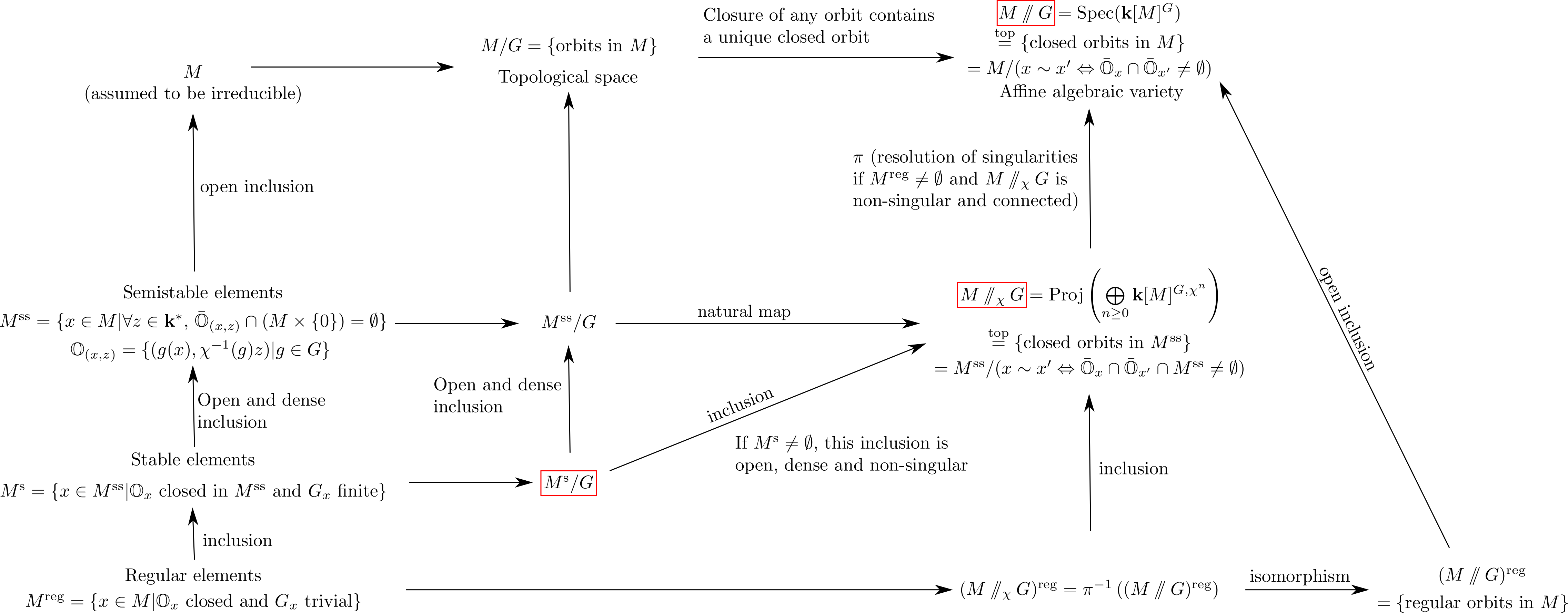
Let $G$ be a reductive linear algebraic group acting algebraically on an affine algebraic variety $M$. We recall that

• Each orbit is a non-singular subvariety of $M$
• For every orbit $\mathbb{O}$, the boundary of $\mathbb{O}$ (i.e. the complement of $\mathbb{O}$ in its closure) is a union of orbits of lower dimension.

Symplectic geometry and Hamiltonian reduction

On any symplectic manifold $M$ (i.e. such that there is a 2-form $\omega \in \Omega^2(M)$ which is closed and non-degenerate), there is a notion of skew-gradient. Indeed, for any function $f$ on $M$ (more properly, we should say that $f$ is a local section of the structure sheaf of $M$), there is a unique vector field $X_f$ such that $\omega (\cdot , X_f) = \mathrm{d}f$. This is analogous to the standard definition of the gradient, but using the symplectic form instead of the metric.

Any symplectic manifold is a Poisson manifold, i.e. we can define a Poisson bracket between functions on $M$. This is done through the skew-gradient construction. Recall that a Poisson bracket is a bilinear antisymmetric morphism $\{\cdot , \cdot \} : \mathcal{O}_M \times \mathcal{O}_M \rightarrow \mathcal{O}_M$ (where $\mathcal{O}_M$ is the structure sheaf, which we identify here to its local sections) which satisfies the Jacobi identity and the Leibniz derivation property. Here, the Poisson bracket is given by $\{f,g\} = \omega (X_f , X_g)$.

Let $M$ be a symplectic manifold and let $G$ be an appropriate¹ Lie group acting on $M$ and preserving the symplectic form. An element $a \in \mathfrak{g}$ defines a vector field $\xi_a$ on $M$, and this vector field preserves $\omega$ (in the sense that the Lie derivative of $\omega$ with respect to $\xi_a$ vanishes). One can show that locally, such a vector field is always the skew-gradient of some function. So there exist functions $H_a$, called the Hamiltonians, such that $\xi_a = X_{H_a}$. We would like to define a "good situation" in which the Poisson bracket of the Hamiltonians and the Lie bracket in the Lie algebra correspond to the same operation, and where the Hamiltonians $H_a$ depend linearly on $a \in \mathfrak{g}$. When we are in this good situation, we say that the action of $G$ is Hamiltonian.

To formalize this, we will introduce the key concept of moment map. More precisely, we say that a symplectic action of $G$ on $M$ is Hamiltonian if there exists a $G$-equivariant map $\mu : M \rightarrow \mathfrak{g}^\ast$, called the moment map, such that

• The Hamiltonian of the vector field $\xi_a$ is given by $H_a(x) = \langle \mu(x),a \rangle$;
• For any $a,b \in \mathfrak{g}$, $\{H_a , H_b \} = H_{[a,b]}$.

A very important example of Hamiltonian action is given by the action of the cotangent bundle. Let $X$ be a manifold with an action of $G$. Then the corresponding action on $T^{\ast}X$ is Hamiltonian, the moment map being given by $\langle \mu (x,\lambda) , a \rangle = \langle \lambda , \xi_a (x) \rangle$, for $x \in X$, $\lambda \in T_x^\ast X$ and $a \in \mathfrak{g}^\ast$. In that case, if we assume furthermore that the action of $G$ is free, then $\mu^{-1}(0)/G$ is a smooth manifold, called the (a) Hamiltonian reduction, and by a theorem of Mardsen and Weinstein, the space $\mu^{-1}(0)/G$ has a canonical structure of a symplectic manifold, inherited from $T^{\ast}X$. We then have the symplectomorphism $$T^{\ast}(X/G) = \mu^{-1}(0)/G \, . $$

Resolutions

Now we want to combine the concepts of the two previous sections, namely GIT and Hamiltonian reductions. The problem is natural: how to generalize the construction of the Hamiltonian reduction $\mu^{-1}(0)/G$ when the action of $G$ is not free, and therefore $\mu^{-1}(0)/G$ is not smooth? We will use GIT. Define $$\mathcal{M}_0 = \mu^{-1}(0) // G \, , \qquad \mathcal{M}_\chi = \mu^{-1}(0) //_{\chi} G \, $$ for a character $\chi : G \rightarrow \mathbf{k}^{\ast}$.

Then one can prove that for any $\chi$, $\mathcal{M}_\chi$ has a Poisson structure, and the morphism $\pi : \mathcal{M}_\chi \rightarrow \mathcal{M}_0$ is a Poisson morphism and a resolution of singularities.

Reference

[1] Kirillov, Quiver representations and quiver varieties. Vol. 174. American Mathematical Soc., 2016.

The Poincaré disk

First of all, I recall that there is a version of the hyperbolic plane that has the shape of a disk. To see that, define the complex coordinate $z=x+iy$, and define the new complex coordinate $u$ by the relation $$iu = \frac{1+iz}{1-iz} \qquad \Leftrightarrow \qquad iz = \frac{-1+iu}{1+iu} \, . $$ It is easy to check that this establishes a bijection between $\mathbb{H}$ parametrized by $z$ and the Poincaré disk $$\mathbb{D} = \{ u \in \mathbb{C} \mid |u|<1 \} \, . $$ The metric on the hyperbolic plane and the Poincaré disk in complex coordinates are \begin{equation} \label{met1} \mathrm{d} s^2_{\mathbb{H}} = \frac{\mathrm{d} z \mathrm{d} \bar{z}}{(\mathrm{Im} \, z)^2} = \frac{4 \mathrm{d} u \mathrm{d} \bar{u}}{(1-|u|^2)^2} \, . \end{equation} One can check that the Ricci scalar is constant and equal to $R=-2$ (obviously, this can be computed in any of the three models).

Embedding in Minkowski space

Now consider the upper sheet of a hyperboloid in Minkowski space $\mathbb{R}^{1,2}$. The metric on this space is $\mathrm{d} s^2_{\textrm{Mink}} = -\mathrm{d} X_0^2 + \mathrm{d} X_1^2 + \mathrm{d} X_2^2$, and the hyperboloid sheet is defined by the equation $$X_0^2 - X_1^2 - X_2^2 = 1 \, , \qquad X_0>0 \, . $$ We can parametrize this by two angles $\alpha$ and $\beta$: \begin{eqnarray*} X_0 &=& \cosh \alpha \\ X_1 &=& \sinh \alpha \cos \beta \\ X_2 &=& \sinh \alpha \sin \beta \end{eqnarray*} Using these coordinates, we find that the metric on the sheet is \begin{equation} \label{met2} \mathrm{d} s^2_{\mathbb{H}} = \mathrm{d} \alpha ^2 + (\sinh \alpha)^2 \mathrm{d} \beta^2 \, , \end{equation} and again we can compute the Ricci scalar and find $R=-2$. The relation between this model and the Poincaré disk model is given by a stereographic projection. More precisely, the Poincaré disk is the stereographic projection of the hyperboloid sheet on the plane $X_0=0$ with respect to the point $(X_0,X_1,X_2)=(-1,0,0)$.

Embedding in Euclidean space

We have just seen that it is possible to embed isometrically the full hyperbolic plane into Minkowski space. Is it possible to do the same in Euclidean space? By this, I mean to find a (regular) map $f : \mathbb{H} \longrightarrow \mathbb{R}^3$ such that the metric induced on the image of $f$ by the Euclidean metric $\mathrm{d} s^2_{\textrm{Eucl}} = \mathrm{d} X_0^2 + \mathrm{d} X_1^2 + \mathrm{d} X_2^2$ be, possibly up to a change of coordinates, the metric $\mathrm{d} s^2_{\mathbb{H}}$ considered in the previous paragraphs. We will see in a minute that the answer is no. In fact, the hyperbolic plane is simply "too big" for $\mathbb{R}^3$. However, if we pick a constant $c>0$ and remove the part of $\mathbb{H}$ that satisfies $y < c$, then a solution is available. Because of a problem of universal covering, we also have to take a part of $\mathbb{H}$ of width $2 \pi c$ in the $x$ direction, for instance $0 \leq x < 2 \pi c$. Then, define $t=\mathrm{ArcCosh} \frac{y}{c}$ and \begin{eqnarray*} X_0 &=& t - \tanh t \\ X_1 &=& \mathrm{sech} \, t \cos \frac{x}{c}\\ X_2 &=& \mathrm{sech} \, t \sin \frac{x}{c} \end{eqnarray*} A cumbersome computation shows that the metric induced on that surface is indeed $\mathrm{d} s^2_{\mathbb{H}}$. This surface is called a (half) pseudosphere. Here is a picture (taken from wikipedia)

So, as we see, it is possible to embed part of the hyperbolic plane in Euclidean $\mathbb{R}^3$. But if you want to embed all of it, this is simply not possible, by a theorem of Hilbert that says that there exists no complete regular surface of constante negative (Gaussian) curvature immersed in $\mathbb{R}^3$. However, for the curvature to be defined, you need to be able to differentiate at least twice on the manifold - this is hidden in the word "regular". To be more precise, a theorem of Efimov tells you that there is no $C^2$ embedding of a complete surface in $\mathbb{R}^3$ with curvature satisfying $K<-\epsilon$ for some strictly positive constant $\epsilon$. But if you're satisfied with a $C^1$ embedding, then the Nash-Kuiper theorem tells you that a $C^1$ isometric embedding of the full hyperbolic plane in Euclidean $\mathbb{R}^2$ does exist! And things become even more counter-intuitive when you know that this embedding can be put inside a ball of arbitrarily small size...

PS : I used this post to answer a question here.

I will describe the theory and the results first, and then illustrate with some examples. I follow closely the textbook by Kirillov [1].

Simple and Indecomposable representations

There are basic operations one can perform on quiver representations. For instance, if two representations $V$ and $W$ are given, we can build their direct sum $V \oplus W$ by summing at each vertex the corresponding vector spaces, and defining the linear maps in the obvious way. Similarly, one can define the concept of subrepresentation. Using this, we have the standard terminology: a representation is

• simple (or irreducible) if it contains no nontrivial subrepresentation,
• semisimple if it is isomorphic to a direct sum of simple representations,
• indecomposable if it cannot be written as a direct sum of nonzero subrepresentations.

A final remark before we proceed: let $V$ be a representation, and let $V=W^0 \supset W^1 \supset \dots \supset W^n=\{0\}$ be a composition series, i.e. a filtration such that all the successive quotients are simple. Then we define the semisimplification of $V$ by $$V^{\mathrm{ss}} = \bigoplus W^n / W^{n+1} \, . $$ This is semisimple, and does not depend on the choice of composition series (by the Jordan-Hölder theorem).

Dynkin Quivers and Gabriel's Theorem

In the study of group or algebra representations, we usually pay much attention to the dimension (this is sometimes even used as a name for the representations, particularly in the physics literature). For a quiver representation $V$, we can do the same, and construct the vector $\mathbf{v} = \mathbf{dim} \, V \in \mathbb{Z}^I$, which contains the dimensions of the various spaces at the various vertices.

Now, given two representations $V$ and $W$ and their dimension vectors $\mathbf{v}$ and $\mathbf{w}$, we can construct a bilinear form $$ \langle \mathbf{v} , \mathbf{w} \rangle = \sum\limits_{i \in I} \mathbf{v}_i \mathbf{w}_i - \sum\limits_{h \in \Omega} \mathbf{v}_{s(h)} \mathbf{w}_{t(h)} \, . $$ This bilinear form has a homological interpretation as $$ \langle V , W \rangle =\sum\limits_{i} (-1)^i \mathrm{dim} \, \mathrm{Ext}^i(V,W) \in \mathbb{Z} \, , $$ but we will not make use of that here. We then introduce the quadratic form $q_{\vec{Q}}(\mathbf{v}) = \frac{1}{2}\langle \mathbf{v} , \mathbf{v} \rangle$, called the Tits form. Note that it is independent of the orientation of the edges, and depends only on the underlying graph $Q$.

With all these preliminary definitions, we can now introduce a particular class of quivers. We say that a connected graph $Q$ is Dynkin if the associated Tits form is positive definite. The reason for this terminology is that a connected graph is Dynkin if and only if it is an ADE Dynkin diagram. A quiver with a Dynkin graph will be called a Dynkin quiver.

The previous result is interesting but not too surprising, given the construction of Dynkin diagrams. What would be more exciting would be a connection with the representation theory of the underlying Lie algebra. As we will see, such a connection exists. First, we introduce yet another definition: we say that the quiver $\vec{Q}$ is of finite type if for any $\mathbf{v} \in \mathbb{Z}_+^I$, the number of isomorphism classes of indecomposable representations of dimension $\mathbf{v}$ is finite. We also denote by $K(\vec{Q})$ the Grothendieck group of the abelian category of representations of $\vec{Q}$; in this group, which is generated by the symbols $[A]$ for $A$ a representation, we have $[A]=[B]$ if $A$ and $B$ are isomorphic, and $[A \oplus B] = [A] + [B]$. This is the appropriate tool to study isomorphism classes of representations. One of the main results of quiver representation theory is Gabriel's theorem:

I will not give the proof here, rather I will try to show the theorem at work on two simple examples.

Examples

Cyclic quiver with one node

Let's take as a first example the quiver with only one vertex, and one arrow having source and target this vertex. This is not a Dynkin quiver, of course. A representation of this quiver is a pair $(V,x)$ where $V$ is a finite-dimensional vector space, and $x$ is an endomorphism of $V$. Classifying these representations is therefore equivalent to classifying matrices up to conjugation. If the base field is (infinite and) algebraically closed, the classification is given by the Jordan form of the matrix. We see that in that case, the number of isomorphism classes of indecomposable representations is infinite.

The $A_2$ quiver

Now let's take the quiver with two nodes linked by one arrow. A representation is given by two vector spaces $V_1$ and $V_2$ and one linear operator $x : V_1 \rightarrow V_2$. By a change of basis, the operator can be brought to the form $$x = \left( \begin{array} I_{r \times r} & 0 \\ 0 & 0 \end{array} \right) \, ,$$ where $I_{r \times r}$ is the unit $r \times r$ matrix. This means that any representation is (isomorphic to) a direct sum of representations of the type $1 : k \rightarrow k$ and $0 : k \rightarrow k$. Let's analyze these two representations:

• The representation $0 : k \rightarrow k$ is actually semisimple, it can be decomposed as the sum of the two simple representations $0 : k \rightarrow 0$ and $0 : 0 \rightarrow k$. These are the representations that we called $S(1)$ and $S(2)$ above.
• The representation $1 : k \rightarrow k$ is not simple (because it is not of the type $S(i)$), indeed it contains $0 : k \rightarrow 0$ as a subrepresentation. Clearly it is not semisimple, but it is indecomposable.

Reference

[1] Kirillov, Quiver representations and quiver varieties. Vol. 174. American Mathematical Soc., 2016.

The classification

The authors focus here on the Coulomb branch (CB), and for simplicity they restrict their attention to the rank 1 case, by which they mean that the CB has complex dimension 1. The classification proceeds in two steps.

1. First, determine the geometries that can be a CB. As shown by Seiberg and Witten a long time ago, the CB can contain singularities, where the theory has additional massless states. If the theory is conformal, the geometry must be scale invariant, and this implies that
   • There can be at most one singular point.
   • Any component of the CB is a flat cone, with deficit angle $\delta$.
   • The singular point, which is the tip of the cone, represents the conformal vacuum (while other points are vacua where conformal invariance is spontaneously broken).
   • Supersymmetry implies that the CB is special Kähler.
   An assumption is added:
   • The CB is supposed to be freely generated, so the CB geometry is "planar" (the complex structure is that of $\mathbb{C}$).
   Using these assumptions, the conical geometries have been classified by Kodaira, and there are seven possibilities, called $II^*$, $III^*$, $IV^*$, $I_0^*$, $IV$, $III$ and $II$, each corresponding to a finite deficit angle $0 < \delta < 2\pi$. In addition, one should mention the singularities $I^*_n$ and $I_n$ with deficit angle $2 \pi$ chich correspond to cusps and are not scale invariant. In the Table below, taken from [1], we see indeed a scale $\Lambda$ in the equation of the curve in those cases.
   
   
2. The second step is to identify the possible $\mathcal{N}=2$ deformations of the CB geometry, which split the singularity. The physical reason for that is that several SCFTs can have the same CB geometry, but different (mass) deformations (for instance, $\mathfrak{su}(2)$ gauge theory with 4 flavors and $\mathfrak{su}(2)$ gauge theory with adjoint matter have the same CB geometry, but distinct mass deformations).
   
   The crucial point here is to take into account the restrictions imposed by supersymmetry on the possible deformations. The authors make and motivate several assumptions that I don't discuss here, and obtain a final list of 28 geometries, as reproduced here from [1]:
   
   

A priori, the classification strategy given above can fail at different points:

• A given CB geometry can correspond to no SCFT ("non-existence")
• A given CB geometry can correspond to several SCFTs, which for instance differ only in their spectrum of irrelevant operators ("non-unicity").

Non freely-generated CBs

The classification of [1] given in the previous paragraph makes the crucial assumption that the CB is holomorphically isomorphic to $\mathbb{C}$, or equivalently that the CB is freely-generated. In [2], the authors examine what happens if this assumption is dropped, finding new internally consistent theories.

The most general CB geometry for an $\mathcal{N}=2$ SCFT is a bouquet of $N$ cones sharing a common tip. We have $$N>1 \Longrightarrow \mbox{The CB is not freely-generated} \, . $$ Under deformation, the CB becomes a non-compact genus $g$ Riemann surface with metric singularities (indicated as before by red dots, image taken from [2]):

Unitarity requires the scaling dimension of scalar operators to be $\geq 1$, and when the CB coordinate $u$ is the vev of such an operator, this translates into $\Delta (u) \geq 1$. But in presence of relations among the CB chiral ring generators, the coordinate is generically not the vev of an operator in the spectrum, and the bound no longer holds. When the constraint $\Delta (u) \geq 1$ is dropped, there are many more scale invariant conical geometries (Table taken from [2]):

Now we have infinite families parametrized by $m \in \mathbb{N}$, and when $m>0$ the singularities are said to be of irregular type.

The main result of [2] is that SCFTs with non-freely-generated rank 1 CBs flow to exotic fixed point theories with non-freely-generated CB chiral rings, and therefore form a closed subset of $\mathcal{N}=2$ theories under RG flow. This might explain why these have not been encountered until recently.

Disconnected Gauge Groups

Finally, in [3] the authors look at what happens when gauging a discrete subgroup of symmetry in 4d $\mathcal{N}=2$ theories from the classification above. In that work, a CB geometry is denoted $[K,F]$ where $K$ is the Kodaira type, and $F$ is the flavor symmetry given in the Table above. Also, one indicates the presence of a chiral deformation parameter of scaling dimension $\delta$ by $\chi_{\delta}$. Then, one can gauge discrete automorphisms of the symmetry $F$. For instance, the theory $[I_0^*,D_4 \chi_0]$ (which is nothing but the $\mathfrak{su}(2)$ theory with 4 flavors) gives birth, gauging a $\mathbb{Z}_2$, to a theory $[III^*,B_3]$, and gauging a $\mathbb{Z}_3$ to $[II^*,G_2]$. Then one can study the RG flows between these theories, and obtain the following Table, taken from [3]:

In many cases, the gauging of the discrete symmetry must be combined with an appropriate gauging of R-symmetry and $SL(2,\mathbb{Z})$ transformation in order to preserve $\mathcal{N}=2$ supersymmetry. Note that a given geometry can appear several times in the Table, this just means, as noted previously, that a given CB geometry can correspond to different theories (and in this case, it can correspond to a parent theory and a daughter theory).

Importantly, as far as I understand, all this discrete gaugings are still holomorphically equivalent to $\mathbb{C}$, and therefore freely-generated. In that sense, it is something different than what is done in [4].

References

[1] Philip Argyres, Matteo Lotito, Yongchao Lü, Mario Martone, Geometric constraints on the space of N=2 SCFTs I: physical constraints on relevant deformations, arXiv:1505.04814

[2] Philip C. Argyres, Yongchao Lü, Mario Martone, Seiberg-Witten geometries for Coulomb branch chiral rings which are not freely generated, arXiv:1704.05110

[3] Philip C. Argyres, Mario Martone, 4d $\mathcal{N}=2$ theories with disconnected gauge groups, arXiv:1611.08602

[4] Antoine Bourget, Alessandro Pini, Diego Rodriguez-Gomez, The Importance of Being Disconnected, A Principal Extension for Serious Groups, arXiv:1804.01108

We consider scattering of $n$ massless particles in arbitrary space-time dimensions, having momentum $p_i^{\mu}$ ($i=1 , \dots , n$) satisfying $p_i^2=0$ and $\sum p_i^{\mu} = 0$. From these, we construct the scattering map $$p^{\mu}(z) = \sum\limits_{i=1}^n p_i^{\mu} \prod\limits_{i \neq j} (z - \sigma_i)$$ where the $\sigma_i$ are fixed by the requirement that $p^2(z)=0$ for all $z$. One can see that $p^{\mu}(z)$ is a degree $n-2$ polynomial in $z$, so $p^2(z)$ has degree $2n-4$. It would seem that this imposes $2n-3$ conditions, but note that $p^2(\sigma_i)=0$ is automatic, so really there are $n-3$ constraints. These constraints are for all $i$: $$E_i := \sum\limits_{j \neq i} \frac{p_i \cdot p_j}{\sigma_i - \sigma_j} = 0 \, , $$ which are called the scattering equations (only $n-3$ of them are independent). The $-3$ here accounts for the $SL(2,\mathbb{C})$ symmetry of the scattering equations: we can fix three of the $\sigma_i$ as we want, and then the other $n-3$ are fixed up to permutation, leaving $(n-3)!$ solutions.

The scattering map contains the information about the $p_i^{\mu}$, which can be recovered using $$p_i^{\mu} = \frac{1}{2 \pi i} \oint_{\sigma_i} \frac{p^{\mu}(z)}{\prod\limits_{j=1}^n (z - \sigma_j)} \, . $$ This is a triviality, but the interesting part comes now. The Cachazo-He-Yuan formula states that the tree-level $n$-particle scattering amplitude of massless theories is given by $$\mathcal{A}_n = \int \mathrm{d} \mu_n \, \mathcal{I}_L \mathcal{I}_R$$ where $\mathcal{I}_L$ and $\mathcal{I}_R$ are factors that depend on the theory under consideration, and $$\mathrm{d} \mu_n = \delta (\sum p_i^{\mu}) \frac{\prod \delta(p_i^2) \prod ' \delta (E_i) \prod \mathrm{d} \sigma_i}{\mathrm{Vol} SL(2, \mathbb{C})} \, . $$ In other words, the measure is an integration over the $\sigma_i$ taking into account all the kinematic constraints given above (the prime indicates that only $n-3$ constraints should be considered out of the $n$ $E_i$). We stress that this is valid in any space-time dimension.

Four dimensions

Now let's look at the four-dimensional case. The crucial observation here is that if $p^{\mu}$ is such that $p^2=0$, then one can use spinorial indices $p^{\mu} \rightarrow p^{\alpha \dot{\alpha}} = \sigma^{\alpha \dot{\alpha}}_\mu p^{\mu}$, and decompose the momentum using two spinors, $$p^{\alpha \dot{\alpha}} = \lambda^{\alpha} \tilde{\lambda}^{\dot{\alpha}} \, . $$ This is valid for all the $p_i^{\mu}$, and also for $$p^{\mu} (z) \rightarrow p^{\alpha \dot{\alpha}}(z) = \rho^{\alpha}(z) \tilde{\rho}^{\dot{\alpha}}(z) \, . $$ In this last equality, the degree $n-2$ can be shared in different ways between $\rho$ and $\tilde{\rho}$ : let's say the degrees are respectively $d$ and $n-2-d$. In that case we say we are in the $d$th sector. We can then parametrize the scattering map using the $d+1$ coefficients $\rho^{\alpha}_k$ of $\rho^{\alpha}$ and the $n-d-1$ coefficients $\tilde{\rho}^{\dot{\alpha}}_k$ of $\tilde{\rho}^{\dot{\alpha}}$. We then introduce a measure $$ \mathrm{d}\mu_{n,d}^{4D} \sim \prod \mathrm{d} \sigma_i \prod \mathrm{d}^2 \rho_k \prod \mathrm{d}^2 \tilde{\rho}_k \, , $$ where the $\sim$ means that I ommit a bunch of delta function and other scalar factors. The CHY measure is then recovered by summing over the sectors. For instance, amplitudes in $\mathcal{N}=4$ SYM decompose as $$\mathcal{A}^{\mathcal{N}=4}_n = \sum\limits_{d=1}^{n-3} \mathcal{A}^{\mathcal{N}=4}_{n,d} \, . $$ I do not explain here how the partial amplitudes $ \mathcal{A}^{\mathcal{N}=4}_{n,d}$ are computed, but note that the $d$th sector has $n-2-2d$ units of helicity violation.

Six dimensions

Let's now turn briefly to six dimensions. The little group was $U(1)$ in four dimensions, and is now $\mathrm{Spin}(4) \sim SU(2) \times SU(2)$. This means that a similar decomposition of $p^{\mu}$ will take place, but with more redundancy. Introducing an angle bracket $\langle \rangle$ taking care of little-group indices contractions, we can write $$p^{AB}(z) = \langle \rho^A(z) \rho^B(z) \rangle$$ with $A,B = 1,2,3,4$. In the case where $n$ is even and the two polynomials above have the same degree, we can obtain an analog of the sector with no helicity violation measure, $\mathrm{d} \mu^{6D}_{n \, \textrm{even}}$. The case of odd $n$ is quite different, in part because this sector does not exist. The details are the object of the paper cited in the introduction.

Considérons une courbe plane fermée de classe $C^1$ et de longueur $1$, paramétrée par sa longueur d'arc, $$\gamma : \mathbb{R}/\mathbb{Z} \rightarrow \mathbb{C} \qquad \textrm{avec} \qquad \forall t \in \mathbb{R}/\mathbb{Z}, \, |\gamma ' (t)| = 1 \, . $$ Pour simplifier, on suppose que la courbe ne s'auto-intersecte pas. Pour calculer l'aire circonscrite par cette courbe on peut utiliser la jolie formule de Stokes, $$\int_{\partial \Omega} \omega = \int_{\Omega} \mathrm{d} \omega$$ où ici $\Omega$ désigne la partie du plan circonscrite par la courbe, qui est donc $\partial \Omega$, et $\omega$ est une 1-forme. On veut que $\mathrm{d} \omega$ soit la forme volume $\mathrm{d} \omega = \mathrm{d} x \wedge \mathrm{d} y$, donc on choisit par exemple $\omega = \frac{1}{2}(x \mathrm{d} y - y \mathrm{d} x)$. Par conséquent, l'aire délimitée par la courbe vaut $$A = \frac{1}{2} \int_{\partial \Omega} (x \mathrm{d} y - y \mathrm{d} x) = \frac{1}{2} \int_{\partial \Omega} (x \mathrm{d} y - y \mathrm{d} x) = \frac{1}{2} \mathrm{Im} \int \gamma '(t) \overline{\gamma (t)} \mathrm{d} t \, . $$ On peut calculer ceci en utilisant les coefficients de Fourier de $\gamma$ et $\gamma'$, donnés par $$c_n = \int e^{- 2 i \pi n t } \gamma(t) \mathrm{d} t \qquad \textrm{et} \qquad c'_n = 2 i \pi n c_n \, . $$ On obtient $$A = \sum\limits_{n \in \mathbb{Z}} \pi n |c_n|^2 \, . $$ D'autre part, la longueur de la courbe vaut (en utilisant $1=|\gamma'| = |\gamma'|^2$) $$1 = \int |\gamma'(t)|^2 \mathrm{d} t = \sum\limits_{n \in \mathbb{Z}} 4 \pi^2 n^2 |c_n|^2 \, . $$ On en déduit que $$A = \sum\limits_{n \in \mathbb{Z}} \pi n |c_n|^2 \leq \sum\limits_{n \in \mathbb{Z}} \pi n^2 |c_n|^2 = \frac{1}{4 \pi} \, , $$ avec égalité si et seulement si les seuls coefficients de Fourier non nuls sont $c_0$ et $c_1$, auquel cas $$\gamma (t) = c_0 + c_1 e^{2 \pi i t} $$ correspond à un cercle, avec $1 = 4 \pi^2 |c_0|^2$, autrement dit un cercle de rayon $\frac{1}{2 \pi}$, qui a bien pour périmètre $1$ et pour aire $\frac{1}{4 \pi}$. L'inégalité isopérimétrique est démontrée.

1. Repérer les pièces non protégées, et regarder comment il est possible de les attaquer.
2. Rechercher les possibles attaques doubles :
   • Les fourchettes (de pions, de Cavalier, de Fous, etc. )
   • Les attaques tout en donnant un échec
   • Les attaques doubles suite à une découverte.
3. Regarder les coups donnant un échec, y compris les sacrifices.
4. Regarder les enfermements, en particulier:
   • Enfermement de Dame si celle-ci est à l'étroit (entourée de pièces de sa propre couleur, ou de pièces adverses protégées)
   • Enfermement de Tours (s'il y a des Fous dans les parages, ils sont particulièrement efficaces contre les Tours)
   • Enfermement de Fous, en utilisant les pions (adverses et alliés).
   On voit le principe général, il faut enfermer une pièce avec des pièces de valeur moindre.
5. Chercher les menaces de mat. Cela peut être combiné avec les autres techniques (double attaque, etc). Observer les cases disponibles pour le Roi adverse et tenter de les contrôler pour créer la menace.
6. Observer les alignements, et voir si on peut en tirer profit : enfilade, clouage, découverte.
7. Si les différentes stratégies présentées dans les points précédents échouent à cause d'une protection de pièce, essayer de dévier cette protection.

Je complèterai cette liste au besoin, si j'ai d'autres idées.